Page 142 - 20dynamics of cancer

THEORY II 127

n = 7
0 (a) 4 (e)
Incidence 1 2 LLA 3 2

3 1
0
0 (b) 4 3 (f)
Incidence 1 2 LLA 2

3 1
0
0 (c) 4 (g)
Incidence 1 2 LLA 3 2

3 1
0
0 (d) 4 (h)
Incidence 1 2 LLA 3 2

3 1
0
20 40 80 20 40 80
Age

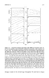
Figure 7.5 Comparison between genotypes with different transition rates. (a-
d) The left incidence panels show the standard log-log plot, with incidence on
a log 10 scale. The bottom, short-dash curve in each incidence panel illustrates
the wild-type genotype. The four incidence curves above the wild type show,
from bottom to top, increasing transition rates between stages. The transition
rate for the bottom curve is u, and for the curves above δu, with δ = 6 i/4 for
i = 1,..., 4. (e-h) The ΔLLA plots on the right show the slope of R, which is the
difference between wild-type and mutant genotypes in the slopes of the log-log
incidence plots calculated from Eq. (7.6). For example, the solid line in each
right panel illustrates the difference in the slopes between the lowest wild-type
curve and the solid curve; each line type on the right illustrates the difference in
log-log slopes between the wild type and the curve with the matching line type
on the left. Each ΔLLA panel has the same parameters as the panel to the left.
In each case, the value of u is obtained by solving for the transition rate that
yields a cumulative incidence of 0.1 at age 80, where cumulative incidence is
2
0
8
4
given by Eq. (6.5). The values of L from top to bottom are L = 10 , 10 , 10 , 10 .
lineages remain in the initial stage throughout life and have n stages