Page 191 - 20dynamics of cancer

176 CHAPTER 9

Relative probability

0 B/2 B
Individual susceptibility

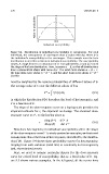
Figure 9.4 Distribution of individual susceptibility to carcinogens. For each
individual, the consequence of carcinogen dose d scales with bd, where b is
the individual’s susceptibility to the carcinogen. This example uses the beta
distribution to describe variation in individual susceptibility. The susceptibility
values, b, range from 0 to a maximum of B. Two parameters, α and β, control
the shape of the beta distribution. Here, I assume α = β, so that all distributions
have a symmetrical shape with mean B/2. The solid curve shows α = β = 1;
the long-dash curve shows α = β = 2, and the short-dash curve shows α = β =
10, 000.
must be weighted by the various probabilities of different values of b.
The average value of S over the different values of b is

∗
S = Sf (b) db, (9.5)
in which the distribution f(b) describes the level of heterogeneity, and
S is a function of b.
The slope of the dose-response curve on a log-log scale provides the
empirical estimate for r, the exponent on dosage. The observed dose-
response curve is S , so the log-log slope is
∗
d log (S ) dS ∗ d
∗
r = = . (9.6)
d log (d) dd S ∗
How does heterogeneity in individual susceptibility affect the shape
of the dose-response curve? To study particular examples, we first need
assumptions about the form of heterogeneity described by the distribu-
tion f(b). Figure 9.4 shows three probability curves for heterogeneity,
ranging from wide variation (solid line) to essentially no heterogeneity
(tall, short-dashed curve).
Next, we need to assume particular shapes for the dose-response
curve for a fixed level of susceptibility, that is, a fixed value of b. Fig-
ure 9.5 shows various examples. In the left panel, all the curves have