Page 178 - 20dynamics of cancer

GENETICS OF PROGRESSION 163

df = 3.0 df = 2.4 df = 2.0
(a) (b) (c)
32
Incidence 16 < 40

40−49
8
50−59
> 60
4 Control
5 4 (d) (e) (f)
Acceleration 3 2 1

-1 0
3 (g) (h) (i)

2
$LLA
1
0
35 45 55 70 35 45 55 70 35 45 55 70
Age

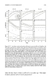
Figure 8.11 Incidence and acceleration of breast cancer in affected families. (a)
This plot is identical to Figure 8.10, with the individual points not shown. Each
curve is derived by fitting a smoothed spline to points at the four ages marked
by ticks on the x axis. In this panel, I used the smooth.spline function of R
with degrees of freedom (df) equal to 3 (R Development Core Team 2004). (b,c)
Incidence curves fit with degrees of freedom equal to 2.4 or 2.0, respectively,
forcing a more linear fit. (d–f) Acceleration, the slope of the incidence curves in
the panels above. The flattening of the acceleration curves near the endpoints
arises at least partly from the spline-fitting procedure, which linearizes the fit
of the incidence curves at the extreme values. (g–i) The differences in the accel-
eration curves from the panels above; each curve is the difference between the
control curve and the curve for one of the groups with an affected relative. Note
that the accelerations are somewhat erratic because they are derived from the
slope of fitted curves based on observations at only four distinct age categories
(see Figure 8.10). By contrast, the ΔLLA values remain relatively stable under
different smoothing stringencies.

when the first-degree relative is affected at an earlier age. Why might
incidence plateau earlier in faster progressors?