Page 172 - 20dynamics of cancer

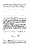
GENETICS OF PROGRESSION 157

assume the other causes of removal happen independently of the event
of interest, we can use the data to estimate a survival curve.
The Kaplan-Meier survival estimate provides the simplest and most
widely used method for lab studies. At each time, t i , at which events
are recorded, the fraction surviving during the interval since the last
recording is σ i = 1−d i /n i , where d i is the number of individuals suffer-
ing an event since the last time of recording at t i−1 , and n i is the number
of individuals at risk during this period. Note that as other causes re-
move individuals, n i decreases over time by more than the number of
observed events. The fraction of individuals that have not suffered an
event (survived) to time t i is the product of the survival fractions over all

time intervals, S(t i ) = σ j , where the product of the σ j ’s is calculated
over all time intervals up to and including t i .
Figure 8.7 shows the steps by which I transform Kaplan-Meier sur-
vival plots (Figure 8.7a) into incidence (Figure 8.7c) and acceleration (Fig-
ure 8.7d) plots. These analytical transformations provide an informative
way of presenting data with regard to quantitative study of progression
dynamics. Frank et al. (2005) give the details for this analysis. Here, I
briefly summarize the main points.
The data in Figure 8.7 come from mouse studies of mutant mismatch
repair (MMR) genotypes. Defects in the MMR system reduce repair of
insertion and deletion frameshift mutations and single base-pair DNA
mismatches (Buermeyer et al. 1999). MMR defects can also reduce initia-
tion of apoptosis in response to DNA damage (Edelmann and Edelmann
2004).
I transformed standard survival plots into incidence by first fitting
a smoothed curve to the survival data (Figure 8.7b). From the survival
curve, S(t), the incidence, measured as probability of death from cancer
per month at age t,is
dS(t) 1 dln (S (t))
I(t) =− =− . (8.4)
dt S(t) dt
I calculated the incidence curves with Eq. (8.4), put incidence and age on
log-log scales, and then fit a straight line through the estimated curves to
get the lines of log-log incidence in Figure 8.7c. I fit straight lines because
the data provide enough information to get a reasonable estimate of the
slope, but not enough information to provide a good estimate of the
curvature of the log-log plots at different ages.