Page 70 - 71 the abc of dft_opt

17.1. PERIMETER PROBLEM 139 140 CHAPTER 17. GRADIENTS

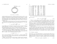
n & local % error GEA % error exact
n=64, eps=0.2
1 0.0 6.2832 0.00 6.2832 0.00 6.2832
1 0.1 6.2832 -0.25 6.2989 0.00 6.2989
1 0.2 6.2832 -1 6.3467 0.01 6.3462
1 0.4 6.2832 -4 6.5455 0.1 6.5371
1 0.8 6.2832 -14 7.5398 3 7.3376
2 0.2 6.2832 -48 6.5371 0.1 6.5297
4 0.2 6.2832 -13 7.2988 1 7.1989
8 0.2 6.2832 -32 10.3455 11 9.2984
16 0.2 6.2832 -57 22.5323 53 14.7104
32 0.2 6.2832 -77 71.2795 166 26.7835
Figure 17.2: Shape r = 1 + 0.2 cos(64 θ). 64 0.2 6.2832 -88 266.2640 400 51.9081

usually be treated by response theory. Perturbation theory will always be accurate once the Table 17.3: Perimeter’s of shapes for * = 0.2, and various n, both exactly and in local approximation and in GEA.
pertubation is sufficiently week, no matter how rapidly the curve is varying (i.e., no matter GEA in this case is
how large n is). The second, less familiar way is when the perturbation is slowly-varying, but GEA loc 1 1 2π 1 dr = 2
<
can be arbitrarily large. This is the case when n is small, but & need not be. In Fig. 17.1, P = P + dθ (17.6)
2 0 r dθ
the local approximation works quite well, even though & is enormous. The ratio of maximum In Table 17.1, we have added the results of the gradient expansion. We see that for
to minimum r is 9!
n = 1, where the local approximation was quite good, GEA reduces the error by at least
Let us first analyze the weak perturbation case. We can cheat by using our knowledge of the
exact functional, but I’m sure there are ways to derive the result without it. If r = r 0 +& f(θ), a factor of 4, and sometimes much more. It also overestimates the perimeter in all cases.
Even up to n = 8, for & = 0.2, the error is still reduced by a factor of 3. But for larger n,
then
= 2 meaning larger gradients, the GEA overcorrects, eventually producing larger errors than the
<
& 2 1 2π df 4
P = 2πr 0 + dθ + O(& ) (17.4) local approximation! Our conclusion is that, for slowly-varying shapes, the gradient expansion
2r 0 0 dθ
greatly improves on the local approximation, but does not work for rapid variations, and can
2
For our standard curve, the integral is n π. There is no linear term, because it vanishes by even worsen the results.
periodicity requirements. You will find this formula quite accurate, even at & = 0.2, and To make the point very clear, suppose we live in a world where most of the shapes we care
hence the (near) quadratic growth in the error in the local approximation in Table 17.1. about have n between 2 and 8, while & varies between .4 and .8. The results of the local and
2
Note that, in the local approximation, there is no & term. Thus the local approximation, gradient expansion approximations are listed in Table ??. Only for the most slowly-varying
while being exact for the circle, is hopeless for weak perturbations around the circle. cases does the GEA really improve over the local approximation. In all cases, it overcorrects,
The other good approximation is called the gradient expansion. We first note that the usually by more than the original error. For these systems, the GEA is hardly an improvement.
only way to make a dimensionless gradient is by dividing the derivative by the radius. We
define s = dr/dθ/r. Then, for a slowly-varying shape, we can write
17.2 Gradient expansion
1 2
P = dθr (1 + C s + . . .) (17.5)
Way back when, in the original Kohn-Sham paper, it was feared that LSD might not be too
where C is yet to be determined. There is no term linear in s, because its integral would good an approximation (it turned out to be one of the most successful ever), and a simple
vanish. Thus the GEA, or gradient expansion approximation, consists of keeping just the first suggestion was made to improve upon its accuracy. The idea was that, for any sufficiently
two terms, once C has been found. slowly varying density, an expansion of a functional in gradients should be of ever increasing
Finding C is easy, once we know the linear response. We simply imagine a perturbation accuracy: 1 ( )
2
3
that is both weak and slow. Then s = dr/dθ/r 0 , and we see that C must be 1/2. Thus the A GEA [n] = d r a(n(r)) + b(n(r))|∇n| + . . . (17.7)