Page 75 - 71 the abc of dft_opt

18.1. FIXING HOLES 149 150 CHAPTER 18. GENERALIZED GRADIENT APPROXIMATION
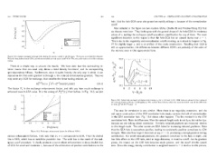
0 hole. But the hole-GGA curve also grows less rapidly at large s, because of the normalization
cutoff.
-0.1 Also included in the figure are two modern GGAs, (Becke 88 and Perdew-Wang 91) that
2πu%n X (u)& -0.2 we discuss more later. They both agree with the general shape of the hole-GGA for moderate
values of s, making the real-space cutoff procedure a justification for any of them. The most
-0.3
He atom significant deviation in this region is that the hole-GGA has an upward bump near s = 1.
-0.4 HF This is due to the negativity and normalization cutoffs meeting, as is about to happen in Fig.
LDA
GGA ?? for slightly larger s, and is an artifact of the crude construction. Recalling that GGA is
-0.5 still an approximation, the differences between different GGA’s are probably of the order of
0 1 2 3
the intrinsic error in this approximate form.
u
Figure 18.2: System-averaged exchange hole density (in atomic units) in the He atom. The exact curve (solid) is Hartree-
Fock, the long dashes denote LDA, and the short dashes are real-space cutoff GGA. The area under each curve is the exchange
energy.
There is a simple way to picture the results. We have seen how the spin-scaling re-
lation means that one need only devise a total density functional, and its corresponding
spin-dependence follows. Furthermore, since it scales linearly, the only way in which it can
depend on the first-order gradient is through s, the reduced dimensionless gradient. Thus we
may write any GGA for exchange, that satisfies the linear scaling relation, as
3
E GGA [n] = 1 d r e unif (n(r))F X (s(r)) (18.1)
X X
The factor F X is the exchange enhancement factor, and tells you how much exchange is
enhanced over its LDA value. It is the analog of F unif (r s ) from before. In Fig. 18.3, we plot
XC
1.8
Figure 18.4: Spherically-averaged correlation hole density n C for r s = 2 and ζ = 0. GEA holes are shown for four values of
1.6 the reduced density gradient, t = |∇n|/(2k s n). The vertical lines indicate where the numerical GGA cuts off the GEA hole
2
to make ! v C dv 4π v n C (v) = 0.
0
F X (s) 1.4
The case for correlation is very similar. Here there is no negativity constraint, and the
Exchange
1.2 hole real-space construction of the GGA correlation hole simply corrects the lack of normalization
GEA in the GEA correlation hole. Fig. 18.4 shows what happens. The line marked 0 is the LDA
B88
PBE correlation hole. Note its diffuseness. Here the natural length scale is not k F u, but rather k s u,
1
0 0.5 1 1.5 2 2.5 3 because we are talking about correlation. Similarly reduced gradients are measured relative
to this length scale. The other curves are GEA holes for increasing reduced gradients. Note
s = |∇n|/(2k F n)
that the GEA hole is everywhere positive, leading to consistently positive corrections to LDA
Figure 18.3: Exchange enhancement factors for different GGA’s
energies. Note also how large it becomes at say t = 1.5, producing a stongly positive energy
various enhancement factors. First note that F X = 1 corresponds to LDA. Then the dashed contribution. For small reduced gradients, the gradient correction to the hole is slight, and
line is GEA, which has an indefinite parabolic rise. The solid line is the result of the real- has little effect on the LSD hole, until at large distances, it must be cutoff. As the gradient
space cutoff procedure. It clearly produces a curve whose enhancement is about double that grows, the impact on the LSD hole becomes much greater, and the cutoff shrinks toward
of GEA for small and moderate s, because of the elimination of positive contributions to the zero. Since the energy density contribution is weighted toward u = 0 relative to this picture,