Page 69 - 71 the abc of dft_opt

138 CHAPTER 17. GRADIENTS

n & local % error exact
1 0.2 6.2832 -1 6.3462
2 0.2 6.2832 -4 6.5297
4 0.2 6.2832 -13 7.1989
Chapter 17 8 0.2 6.2832 -32 9.2984
16 0.2 6.2832 -57 14.7104
32 0.2 6.2832 -77 26.7835
Gradients 64 0.2 6.2832 -88 51.9081

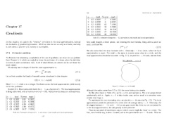
Table 17.2: Perimeter’s of shapes for * = 0.2, and various n, both exactly and in local approximation.
In this chapter, we explore the ”obvious” correction to the local approximation, namely One could imagine a clever person, not knowing the true formula, being able to prove an
the inclusion of gradient information. We’ll see that its not as easy as it looks, and why exact condition like:
it took about a quarter of a century to accomplish. P loc ≤ P (17.3)
We also notice that the error increases with &. Obviously & = 0 is a circle, where the local
17.1 Perimeter problem approximation is exact. For small &, the curve is in some sense close to a circle, and the
local approximation should be accurate. In Fig. 17.1, we plot the & = 0.8 case, and see that,
To illustrate the interesting complexities of the use of gradients, we return to our problem
from Chapter 2, in which we needed to know the perimeter of a shape, given its definition n=1, eps=0.8
in terms of polar coordinates, r(θ). In all of what follows, we assume we do not know the
exact answer.
We already saw in chapter 8 that the local approximation is
1 2π
P loc = dθ r(θ). (17.1)
0
Let us first consider the family of smooth curves introduced in that chapter:

r(θ) = 1 + & cos(nθ) (17.2)
Here 0 ≤ & < 1, while n is an integer. For these curves, the local approximation yields exactly
2π for the perimeter. Figure 17.1: Shape r = 1 + 0.8 cos(θ).
In table 17.1, I have compared results for n = 1, as a function of &. The local approximation although the radius varies from 0.2 to 1.8, the curve looks quite circular.
is doing rather well, with a maximum error of −15%. Notice how its always an underestimate.
On the other hand, in Table 17.1, we fix & = 0.2, and increase n. The error grows almost
quadratically with n. Again, n = 0 is the circular case, and so small n is somehow more
n & local % error exact
circular than large n.
1 0.0 6.2832 0.00 6.2832 To understand the ever increasing error, we plot the n = 64 curve in Fig. 17.2. The local
1 0.1 6.2832 -0.25 6.2989
approximation yields the perimeter of a circle with the average radius, r = 1. Obviously, the
1 0.2 6.2832 -0.99 6.3462
64 wiggles between r = 1.2 and r = 0.8 as one goes round the circle are not accounted for
1 0.4 6.2832 -3.88 6.5371 in the local approximation, but add greatly to the perimeter.
1 0.8 6.2832 -14.37 7.3376
Thus we can speak of two distinct ways in which a curve might be ’close’ to a circle. The
Table 17.1: Perimeter’s of shapes for n = 1, and various *, both exactly and in local approximation. first, more familiar way, is when & is small, and so the perturbation on r = 1 is weak. This can
137