Page 265 - 35Linear Algebra
P. 265

14.5 QR Decomposition                                                                         265


                                   ⊥
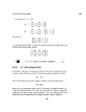
                      First, we set v := v 1 . Then
                                   1
                                                           
                                               1        1       0
                                                        1
                                               1
                                                                0
                                    v ⊥  :=     −  2     =   
                                     2               2
                                               1        0       1
                                                                     
                                               3     4  1     1   0        1
                                    v 3 ⊥  :=     −     −      =   −1   .
                                                                  0
                                               1
                                                        1
                                               1     2  0     1   1        0
                   Then the set
                                                           
                                               1       0       1 
                                                  1  ,  0   ,  −1
                                                            
                                                  0     1       0
                                                                  
                                            3
                   is an orthogonal basis for R . To obtain an orthonormal basis we simply divide each
                   of these vectors by its length, yielding
                                                1         1  
                                                 √       0     √
                                                  2
                                                                  
                                                                2 
                                                  1            −1     .
                                                             
                                                √  , 0 ,  √ 
                                                  2
                                                                2 
                                                  0      1      0
                                                                  
                                      A 4 × 4 Gram--Schmidt Example

                   14.5      QR Decomposition

                   In Chapter 7, Section 7.7 teaches you how to solve linear systems by decom-
                   posing a matrix M into a product of lower and upper triangular matrices


                                                     M = LU .

                   The Gram–Schmidt procedure suggests another matrix decomposition,

                                                    M = QR ,


                   where Q is an orthogonal matrix and R is an upper triangular matrix. So-
                   called QR-decompositions are useful for solving linear systems, eigenvalue
                   problems and least squares approximations. You can easily get the idea
                   behind the QR decomposition by working through a simple example.


                                                                  265
   260   261   262   263   264   265   266   267   268   269   270