Page 77 - 35Linear Algebra

3.3 Dantzig’s Algorithm 77

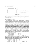
variables (incl. slack and artificial) objective
z }| { z}|{

 
← constraint equations
 
 
 
← objective equation
↑
objective value

Figure 3.1: Arranging the information of an optimization problem in an
augmented matrix.

Example 41 (Performing EROs)
We scan the last row, and notice the (most negative) coefficient −4. Na¨ıvely you
might think that this is good because this multiplies the positive variable w and only
helps the objective function f = 4w + · · · . However, what this actually means is
that the variable w will be positive and thus determined by the constraints. Therefore
we want to remove it from the objective function. We can zero out this entry by
performing a row operation. For that, either of the first two rows could be used.
To decide which, we remember that we still have to solve solve the constraints for
variables that are positive. Hence we should try to keep the first two entries in the
last column positive. Hence we choose the row which will add the smallest constant
to f when we zero out the −4: Look at the last column (where the values of the
constraints are stored). We see that adding four times the first row to the last row
would zero out the −4 entry but add 20 to f, while adding two times the second row
to the last row would also zero out the −4 but only add 12 to f. (You can follow this
by watching what happens to the last entry in the last row.) So we perform the latter
row operation and obtain the following:
 
1 1 1 1 0 5 c 1 = 5
 
1 2 3 2 0 c 2 = 6
 6 
−1 7 7 0 1 12 f = 12 + x − 7y − 7z .
We do not want to undo any of our good work when we perform further row operations,
so now we use the second row to zero out all other entries in the fourth column. This
is achieved by subtracting half the second row from the first:
 
1 0 − 1 0 0 2 c 1 − c 2 = 2
1
2 2 2
 
1 2 3 2 0 c 2 = 6
 6 
−1 7 7 0 1 12 f = 12 + x − 7y − 7z .
77