Page 75 - 35Linear Algebra

3.3 Dantzig’s Algorithm 75

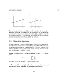
Here we have plotted the curve f(x) = d in the case where the function f is
linear and non-linear. To optimize f in the interval [a, b], for the linear case
we just need to compute and compare the values f(a) and f(b). In contrast,
for non-linear functions it is necessary to also compute the derivative df/dx
to study whether there are extrema inside the interval.

3.3 Dantzig’s Algorithm

In simple situations a graphical method might suffice, but in many applica-
tions there may be thousands or even millions of variables and constraints.
Clearly an algorithm that can be implemented on a computer is needed. The
simplex algorithm (usually attributed to George Dantzig) provides exactly
that. It begins with a standard problem:

Problem 38 Maximize f(x 1 , . . . , x n ) where f is linear, x i ≥ 0 (i = 1, . . . , n) sub-
ject to
 
x 1
.
Mx = v , x :=  .  ,
 . 
x n
where the m × n matrix M and m × 1 column vector v are given.

This is solved by arranging the information in an augmented matrix and
then applying EROs. To see how this works lets try an example.

75