Page 423 - 35Linear Algebra

G.13 Orthonormal Bases and Complements 423

⊥
⊥
⊥
(v · v 4 ) ⊥ (v · v 4 ) ⊥ (v · v 4 ) ⊥
⊥
2
1
3
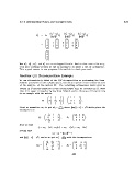
v 4 = v 4 − v − v − v 3
2
1
kv k kv k kv k
⊥ 2
⊥ 2
⊥ 2
1 2 3
       
1 0 0 3
0
1
0
1
  1   0   3  
=   −   −   −  
1 1 9
 0   0   1   0 
2 0 0 0
 
0
0
 
=  
 0 
2
⊥
⊥
⊥
Now v , v , v , and v ⊥ are an orthogonal basis. Notice that even with very,
1 2 3 4
very nice looking vectors we end up having to do quite a bit of arithmetic.
This a good reason to use programs like matlab to check your work.
Another QR Decomposition Example
We can alternatively think of the QR decomposition as performing the Gram-
Schmidt procedure on the column space, the vector space of the column vectors
of the matrix, of the matrix M. The resulting orthonormal basis will be
stored in Q and the negative of the coefficients will be recorded in R. Note
that R is upper triangular by how Gram-Schmidt works. Here we will explicitly
do an example with the matrix
   
1 1 −1
M =  m 1 m 2 m 3  =  0 1 2  .
−1 1 1
√
1
0
First we normalize m 1 to get m = km 1 k where km 1 k = r = 2 which gives the
m 1
1
1
decomposition
√
√ 1 −1
 1  
2 2 0 0
Q 1 =  0 1 2  , R 1 =  0 1 0  .
− √ 1 1 1 0 0 1
2
Next we find
0
0
1
t 2 = m 2 − (m 0 m 2 )m = m 2 − r m = m 2 − 0m 0
1 1 2 1 1
noting that
0
0
2
m 0 1 m = km k = 1
1
1
√
0
2
and kt 2 k = r = 3, and so we get m = t 2 with the decomposition
2 2 kt 2 k
√
 1 1 
√ √ −1 
2 3 2 √ 0 0
Q 2 =  0 √ 1 2  , R 2 =  0 3 0  .


3
1 1
− √ √ 1 0 0 1
2 3
423