Page 413 - 35Linear Algebra
P. 413

G.11 Eigenvalues and Eigenvectors                                                             413


                   degree n polynomials have n complex roots (counted with multiplicity). The
                   word can does not mean that explicit formulas for this are known (in fact
                   explicit formulas can only be give for degree four or less). The necessity
                   for complex numbers is easily seems from a polynomial like
                                                        2
                                                       z + 1
                                                            2
                   whose roots would require us to solve z = −1 which is impossible for real
                   number z. However, introducing the imaginary unit i with
                                                      2
                                                      i = −1 ,
                   we have
                                                 2
                                                z + 1 = (z − i)(z + i) .
                   Returning to our characteristic polynomial, we call on the fundamental theorem
                   of algebra to write
                                         P M (λ) = (λ − λ 1 )(λ − λ 2 ) · · · (λ − λ n ) .

                   The roots λ 1 , λ 2 ,...,λ n are the eigenvalues of M (or its underlying linear
                   transformation L).

                   Eigenspaces

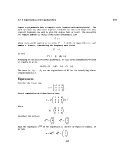
                   Consider the linear map
                                                              
                                                       −4  6  6
                                                 L =   0  2  0   .
                                                       −3  3  5
                   Direct computation will show that we have

                                                              
                                                      −1   0  0
                                               L = Q   0  2  0   Q −1
                                                        0  0  2
                   where
                                                              
                                                        2  1  1
                                                  Q =   0  0  1  .
                                                        1  1  0

                   Therefore the vectors
                                                                 
                                                     1             1
                                              (2)            (2)
                                             v   =   0    v   =   1 
                                              1              2
                                                     1             0
                   span the eigenspace E (2)  of the eigenvalue 2, and for an explicit example, if
                   we take
                                                                  
                                                                  1
                                                    (2)   (2)
                                               v = 2v  − v   =   −1 
                                                    1     2
                                                                  2
                                                                  413
   408   409   410   411   412   413   414   415   416   417   418