Page 48 - 49A Field Guide to Genetic Programming

34 4 Example Genetic Programming Run

(a) (b) (c) (d)

- + - +

+ 0 % 0 x 0 1 *

x 1 x x + x

x 1
2
x+1 1 x x + x + 1

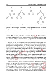
Figure 4.3: Population of generation 1 (after one reproduction, one muta-
tion, and two one-offspring crossover operations).

ation %. The resulting individual is shown in Figure 4.3b. This particular
mutation changes the original individual from one having a constant value
of 2 into one having a constant value of 1, improving its fitness from 17.98
to 11.0.

Finally, we use the crossover operation to generate our final two indi-
viduals for the next generation. Because the first and second individuals in
generation 0 are both relatively fit, they are likely to be selected to partic-
ipate in crossover. However, selection can always pick suboptimal individ-
uals. So, let us assume that in our first application of crossover the pair of
selected parents is composed of the above-average tree in Figures 4.1a and
the below-average tree in Figure 4.1d. One point of the first parent, namely
the + function in Figure 4.1a, is randomly picked as the crossover point for
the first parent. One point of the second parent, namely the leftmost termi-
nal x in Figure 4.1d, is randomly picked as the crossover point for the second
parent. The crossover operation is then performed on the two parents. The
offspring (Figure 4.3c) is equivalent to x and is not particularly noteworthy.

Let us now assume, that in our second application of crossover, selection
chooses the two most fit individuals as parents: the individual in Figure 4.1b
as the first parent, and the individual in Figure 4.1a as the second. Let us
further imagine that crossover picks the leftmost terminal x in Figure 4.1b
as a crossover point for the first parent, and the + function in Figure 4.1a as
the crossover point for the second parent. Now the offspring (Figure 4.3d)
2
is equivalent to x + x + 1 and has a fitness (sum of absolute errors) of zero.