Page 293 - 35Linear Algebra

16.2 Image 293

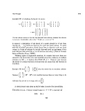
Example 148 of calculating the kernel of a matrix.

     
1 2 0 1 1 2 0 1 1 2 0 1
ker  1 2 1 2  = ker  0 0 1 1  = ker  0 0 1 1 
0 0 1 1 0 0 1 1 0 0 0 0
   
 −2 −1 
 
 
 1   0 
,
= span     .
0
   
 −1 
 
 
0 1
The two column vectors in this last line describe linear relations between the columns
c 1 , c 2 , c 3 , c 4 . In particular −2c 1 + 1c 2 = 0 and −c 1 − c 3 + c 4 = 0.
In general, a description of the kernel of a matrix should be of the form
span{v 1 , v 2 , . . . , v n } with one vector v i for each non-pivot column. To agree
with the standard procedure, think about how to describe each non-pivot
column in terms of columns to its left; this will yield an expression of the
form wherein each vector has a 1 as its last non-zero entry. (Think of Column
Reduced Echelon Form, CREF.)
Thinking again of augmented matrices, if a matrix has more than one
element in its kernel then it is not invertible since the existence of multiple
solutions to Mx = 0 implies that RREF M 6= I. However just because
the kernel of a linear function is trivial does not mean that the function is
invertible.

 
1 0
0
Example 149 ker  1 1  = since the matrix has no non-pivot columns.
0
0 1
 
1 0
3
2
However,  1 1  : R → R is not invertible because there are many things in its
0 1
 
1
codomain that are not in its range, such as  
0 .
0
A trivial kernel only gives us half of what is needed for invertibility.

Theorem 16.2.2. A linear transformation L: V → W is injective iff

kerL = {0 V } .

293