Page 47 - 49A Field Guide to Genetic Programming

4.2 Step-by-Step Sample Run 33

4 4

-1 1 -1 1
(a) (b)
-2 -2

4 4

-1 1 -1 1
(c) (d)
-2 -2

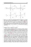
Figure 4.2: Graphs of the evolved functions from generation 0. The solid
2
line in each plot is the target function x + x + 1, with the dashed line
being the evolved functions from the first generation (see Figure 4.1). The
fitness of each of the four randomly created individuals of generation 0 is
approximately proportional to the area between two curves, with the actual
fitness values being 7.7, 11.0, 17.98 and 28.7 for individuals (a) through (d),
respectively.

population will not necessarily be excluded.
In this example we will start with the reproduction operation. Because
the first individual (Figure 4.1a) is the most fit individual in the population,
it is very likely to be selected to participate in a genetic operation. Let us
suppose that this particular individual is, in fact, selected for reproduction.
If so, it is copied, without alteration, into the next generation (generation 1).
It is shown in Figure 4.3a as part of the population of the new generation.
We next perform the mutation operation. Because selection is proba-
bilistic, it is possible that the third best individual in the population (Fig-
ure 4.1c) is selected. One of the three nodes of this individual is then ran-
domly picked as the site for the mutation. In this example, the constant
terminal 2 is picked as the mutation site. This program is then randomly
mutated by deleting the entire subtree rooted at the picked point (in this
case, just the constant terminal 2) and inserting a subtree that is randomly
constructed in the same way that the individuals of the initial random pop-
ulation were originally created. In this particular instance, the randomly
grown subtree computes x divided by x using the protected division oper-