Page 150 - 49A Field Guide to Genetic Programming

136 13 Troubleshooting GP

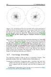
Figure 13.1: Visualisation of the size and shape of the entire population of
1,000 individuals in the final generation of runs using a depth limit of 50 (on
the left) and a size limit of 600 (on the right). The inner circle is at depth
50, and the outer circle is at depth 100. These plots are from (Crane and
McPhee, 2005) and were drawn using the techniques described in (Daida
et al., 2005).

way is to use GP as a multi-objective evolutionary algorithm (cf. Chapter 9.)
In some cases the details of the trees are less important than their general
size and shape. Daida et al. (2005) presented a particularly useful set of
visualisation techniques for this situation. 5 These techniques allow one to
see the size and shape of both individual trees as well as an aggregate view
of entire populations. Figure 13.1, for example, shows the impact of size and
depth limits on the size and shape of trees in two different runs with very
similar average sizes and depths. The plots make it clear, however, that the
shapes of the resulting trees were quite different.

13.7 Encourage Diversity

One important property to keep an eye on is population diversity. Two
particular measures that can be useful sources of information are:
Frequency of primitives Recognising when a primitive has been com-
pletely lost from the population (or its frequency has fallen to a low
level, consistent with the mutation rate) may help to diagnose prob-
lems.
5
A Mathematica implementation of this technique can be downloaded from http:
//library.wolfram.com/infocenter/MathSource/5163/.