Page 372 - 35Linear Algebra

372 Movie Scripts

Any value of µ will give a solution of the system, and any system can be written
in this form for some value of µ. Since there are multiple solutions, we can
also express them as a set:
      
 x 1 2 −3 
 x 2  =  1  + µ  0  µ ∈ R .
 
x 3 0 1
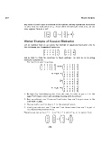
Worked Examples of Gaussian Elimination
Let us consider that we are given two systems of equations that give rise to
the following two (augmented) matrices:
   
2 5 2 0 2 5 2 9
 1 1 1 0 1   0 5 10 
1 4 1 0 1 0 3 6
and we want to find the solution to those systems. We will do so by doing
Gaussian elimination.
For the first matrix we have
   
2 5 2 0 2 1 1 1 0 1
∼
 1 1 1 0 1  R 1 ↔R 2  2 5 2 0 2 
1 4 1 0 1 1 4 1 0 1
 
1 1 1 0 1
R 2 −2R 1 ;R 3 −R 1
∼  0 3 0 0 0 
0 3 0 0 0
 
1 1 1 0 1
1
3 R 2
∼  0 1 0 0 0 
0 3 0 0 0
 
1 0 1 0 1
R 1 −R 2 ;R 3 −3R 2  0
∼ 1 0 0 0 
0 0 0 0 0
1. We begin by interchanging the first two rows in order to get a 1 in the
upper-left hand corner and avoiding dealing with fractions.
2. Next we subtract row 1 from row 3 and twice from row 2 to get zeros in the
left-most column.
3. Then we scale row 2 to have a 1 in the eventual pivot.
4. Finally we subtract row 2 from row 1 and three times from row 2 to get it
into Reduced Row Echelon Form.
Therefore we can write x = 1 − λ, y = 0, z = λ and w = µ, or in vector form
       
x 1 −1 0
0
y
0
     0   
  =   + λ   + µ   .
 z   0   1   0 
w 0 0 1
372